Risk Assessment Surface Methodology

This page describes the methodology behind the WNV risk surface maps. Note that these estimates are derived from the Risk Assessment Model found in the California Mosquito-Borne Virus Surveillance and Response Plan and that other states may use different benchmark values than are described here.

Background

Every Sunday, surfaces are generated for the prior week. For example, if today was the 15th, the prior week would be from the 8th to the 14th. The initial map, i.e. of California, is reduced to a pixelized grid, where each pixel is 1/32 of a degree (approximately 3.5 km). Because the surveillance factors, apart from Environmental Conditions, are for a specific point, all points within a pixel are aggregated for that pixel. For example, if two trap sites from which arthropod abundance was estimated came from within the same pixel, those abundance estimates would be combined for that pixel.

There are five surveillance factors that comprise the risk surface: Environmental Conditions, Arthropod Abundance Anomaly, Viral Infection Rate, Sentinel Chicken Seroconversions, and Dead Bird Infections. Each of these components receives an Assessment Value ranging from 1 (lowest risk) to 5 (highest risk), which are then averaged to create the final Response Level. Human cases do not factor into the risk calculations because they are considered outcome measures.

Surveillance Factors

Environmental Conditions

The Environmental Conditions component of the risk assessment is based on the average daily temperature, which is an average of hourly data. These data come from the NASA North American Land Data Assimilation System, which generates temperature surfaces on a 1/8th-degree grid. To convert to the smaller grid used for the risk assessment surfaces, the temperature from the larger pixel is applied to all smaller pixels within.

The Assessment Values are assigned for the following benchmarks:

1. Average daily temperature ≤ 56 F
2. Average daily temperature > 56 and ≤ 65 F
3. Average daily temperature > 65 and ≤ 72 F
4. Average daily temperature > 72 and ≤ 79 F
5. Average daily temperature > 79 F

Arthropod Abundance Anomaly

The Arthropod Abundance Anomaly component of the risk assessment is derived separately for the two primary WNV vectors, Cx tarsalis and the Cx pipiens complex, and for four trap types, New Jersey light traps, CO₂-baited traps, gravid traps, and resting box traps. For each species and trap type, the total number collected within a pixel is summed and compared to the 5-year average total for the same period. This 5-year average is calculated if the site has at least 2 nonconsecutive years of data in the previous 5 years for the corresponding surveillance week. The pixel’s anomaly value is then interpolated using an inverse-distance weighting process to the pixels that are fully or partially within an 8 km zone of the initial pixel, as long as the pixels centroid point is within the 8 km zone. This results in four surfaces for each species, one surface per trap type. For each final pixel, the set of four corresponding pixels are examined and the value that is closest to the original pixel is chosen to create the final surface for each species. In the case of a tie, the larger abundance anomaly is chosen.

The Assessment Values are assigned for the following benchmarks:

1. Vector abundance well below average (≤ 50%)
2. Vector abundance below average (> 50% and ≤ 90%)
3. Vector abundance average (> 90% and ≤ 150%)
4. Vector abundance above average (> 150% and ≤ 300%)
5. Vector abundance well above average (> 300%)

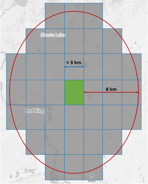
Inverse-distance weighting

The inverse-distance weighting process means that the abundance (or infection rate) value from the original pixel (here reperesented in green) is applied to the surrounding pixels in the buffer zone (represented in gray). The pixels appear elongated farther north due to narrowing of longitude lines near the poles on this map projection.

If there is only one surface, as in the image below, that value is taken to represent the value for each pixel. If two surfaces overlap - i.e. two pixels with abundance observations in the same week are within 8 km of each other, which is common during peak WNV seasons - the value for the pixel that is closest to its original point is taken as the value for that pixel. For example, if a pixel lies within two buffer zones and is 1 unit away from one observation but 2 units away from another observation, the value from the observation 1 unit away is chosen. The maximum value is taken if a pixel is equidistant from two points.

Viral Infection Rate

The Viral Infection Rate component of the risk assessment is also derived separately for the two primary WNV vectors, Cx. tarsalis and the Cx pipiens complex, and for three trap types, CO₂-baited traps, gravid traps, and resting box traps. For each species and trap type, the infection rate per 1000 mosquitoes is calculated for each pixel by dividing the number of positive pools by the number of mosquitoes tested. This value is interpolated using an inverse-distance weighting process in the same manner as the abundance anomaly to the pixels within an 8 km zone of the initial pixel and the final surface is chosen in the same manner as described above.

The Assessment Values are assigned for the following benchmarks:

1. MIR = 0
2. MIR > 0 and ≤ 1.0
3. MIR > 1.0 and ≤ 2.0
4. MIR > 2.0 and ≤ 5.0
5. MIR > 5.0

Sentinel Chicken Seroconversions

The Sentinel Chicken Seroconversions component of the risk assessment is the number of chickens in a flock that develop antibodies to WNV and/or the number of flocks with seropositive chickens. Notably, there are two defined regions the sentinel flocks: the specific region and the broad region. The specific region is the pixel where the flock is located while the broad region represents the pixels ~241 km around the pixel with a flock. Pixels in the broad region do not contribute to the risk surface unless there is overlap with mosquito endpoints.

The Assessment Values are assigned for the following benchmarks:

1. No seroconversions in the broad region.
2. One or more seroconversions in the broad region.
3. One or two seroconversions in a single flock in the specific region.
4. More than two seroconversions in a single flock or two flocks with one or two seroconversions in the specific region.
5. More than two seroconversions per flock in multiple flocks in the specific region.

Dead Bird Infections

The Dead Bird Infections component of the risk assessment is the number of positive dead birds found in a given pixel during the previous four weeks. This longer time period reduces the impact of zip code closures during periods of increased WNV transmission. Similar to the Sentinel Chicken Seroconversions, there are two defined regions for dead bird infections: the specific region and the broad region. The specific region is the pixel where the dead bird was located while the broad region represents the pixels ~241 km around the pixel with a dead bird. Pixels in the broad region do not contribute to the risk surface unless there is overlap with mosquito endpoints.

The Assessment Values are assigned for the following benchmarks:

1. No positive dead birds in the broad region.
2. One or more positive dead birds in the broad region.
3. One positive dead bird in the specific region.
4. Two to five positive dead birds in the specific region.
5. More than five positive dead birds in the specific region.

Risk Surfaces

The final Response level is derived from the average of the five Assessment Values for a given pixel. The response levels fall into three categories:

1. Normal Season (Average rating 1.0-2.5)
2. Emergency Planning (Average rating 2.6-4.0)
3. Epidemic (Average rating 4.1-5.0)

These values are averaged separately for Cx tarsalis and the Cx pipiens complex. For example, in a pixel where the average temperature was 83 F (5), the Cx tarsalis abundance anomaly was 200% (4), the MIR was 2.5 (4), no seroconversions were detected (1), and one positive bird was found (2), the response level would be the average of these values, 3.2, which is considered Emergency Planning.